# Basic Properties of Feedback
# Perspective on the Properties of Feedback
Perspective on the Properties of Feedback A major goal of control is to keep the tracking error ($y_d - y$) small in the face of some parameter changes
– by changing the plant? – by changing the sensor type and location? – by changing the controller? → this course, esp. with feedback
• Feedback can modify: – system stability – response to reference input and disturbances (both predictable/measurable or not) – sensitivity to parameter changes
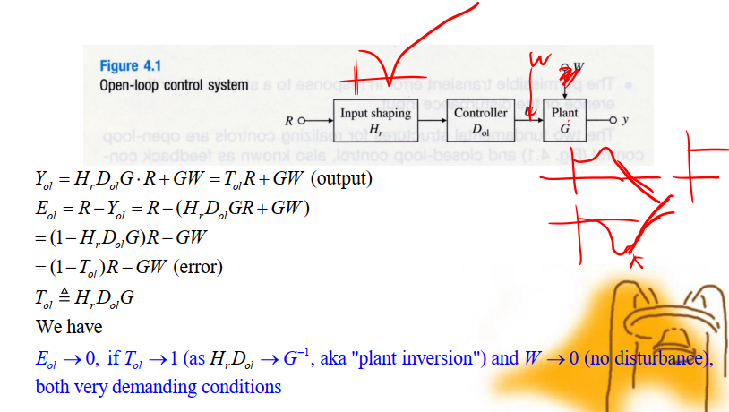
# Open-Loop Control
updt 4
The github file directory:

Example image (source is in content/notes/images/example.png)

# Feedback control
 Pasted image 20230520152418.png

![[Pasted image 20230520152418.png]](https://alexnder77.github.io//./Pastedimage%20230520152418.png)
# Errors due to constant disturbances
Historic case: Watt’s problem of disturbance rejection – steady-state speed of early engines would change substantially when presented with added torque caused by a new load – feedback was introduced by adding a flying ball governor
Pasted image 20230520152507.png
# Sensitivity of System Gain to Parameter Changes
Historic case: Black’s telephone line repeaters for Bell Labs – Electronic components drifting led to amplifier gain drifting – Feedback was introduced to amplifier design
Pasted image 20230520152612.png
# Tradeoff between Tracking Performances and Sensor Noise Rejection with Feedback Control
Pasted image 20230520152651.png
# Definition of System Type
Pasted image 20230520152822.png
# HW 4
# review questions
- Give three advantages of feedback in control.
- Stability: Feedback control can make a system more stable, preventing it from reacting excessively to disturbances.
- Accuracy: Feedback systems can correct for disturbances or errors in the system, thereby improving the accuracy of the output.
- Adaptability: Feedback control systems can adapt to changes in the system’s parameters or the environment, maintaining performance despite these changes.
- Give two disadvantages of feedback in control.
- Complexity: Feedback control systems can be more complex to design and implement compared to open-loop systems.
- Stability Issues: While feedback can enhance stability, improper design of the feedback system can also lead to instability.
A temperature control system is found to have zero error to a constant tracking input and an error of 0.5°C to a tracking input that is linear in time, rising at the rate of 40°C/ sec. What is the system type of this control system and what is the relevant error constant (Kp or Kv or etc.)?
What are the units of Kp, Kv, and Ka?
- Kp (Position error constant): unitless, because it multiplies an error measured in the same units as the system output.
- Kv (Velocity error constant): s^-1 (per second), as it’s the system’s gain against a ramp input (rate of change of output).
- Ka (Acceleration error constant): s^-2 (per second squared), as it represents the system’s gain against a parabolic or acceleration input.
What is the definition of system type with respect to reference inputs? The system type with respect to reference inputs is a classification of control systems based on the number of pure integrators in the system’s open-loop transfer function. Type 0 systems have no integrators, Type 1 systems have one integrator, Type 2 systems have two, and so on. The system type determines the system’s ability to achieve zero steady-state error for various types of reference inputs (step, ramp, etc.).
What is the definition of system type with respect to disturbance inputs? The system type with respect to disturbance inputs is similarly based on the number of pure integrators in the system, but it involves the closed-loop transfer function from the disturbance input to the system output. The system’s ability to reject disturbance inputs is dependent on this type.
Why does system type depend on where the external signal enters the system? The system type depends on where the external signal enters the system because the signal’s path through the system determines how many integrations it undergoes before influencing the system output. The control system may handle reference inputs and disturbance inputs differently because they often enter the system at different points, affecting the resultant closed-loop transfer function. For example, a reference input is typically applied at the system’s input, while a disturbance might be introduced at various points within the system.
# 4.2
Pasted image 20230604204549.png
a) (a) $$\frac{Y}{R}=-\beta_1 K^3 \Longrightarrow \beta_1=0.01 $$ (b) $$ \frac{Y}{R}=\left(\frac{-K}{1+\beta_2 K}\right)^3 \Longrightarrow \beta_2=0.364 $$ (c) $$ \frac{Y}{R}=\frac{-K^3}{1+\beta_3 K^3} \Longrightarrow \beta_3=0.099$$
b) Sensitivity $S_K^G, \quad G=\frac{Y}{R}$ (a)
$$ \begin{gathered} \frac{d G}{d K}=-3 \beta_1 K^2 \\ \mathcal{S}_K^G=\frac{K}{G} \frac{d G}{d K}=\frac{K}{-\beta_1 K^3}\left(-3 \beta_1 K^2\right)=3 \end{gathered} $$
(b)
$$ S_K^G=0.646 $$

(c)
$$S_K^G=0.03$$
Case $c$ is the least sensitive.
c) Sensitivities w.r.t. feedback gains:
(b) $$ \mathcal{S}_{\beta_2}^G=-2.354 $$
(c) $$ \mathcal{S}_{\beta_3}^G=-0.99 $$
# 4.22
Pasted image 20230604204452.png a) Pasted image 20230604210256.png b) If $V_a=$ constant the system is in steady state: $$ \dot{\theta}=\frac{b_0}{a_1} V_a=\frac{200 \times 100}{65} \frac{60}{2 \pi} \frac{\mathrm{rad} . s e c^{-1}}{\mathrm{rpm}}=2938 \mathrm{rpm} $$ (c) $$ \begin{aligned} \frac{\theta}{\theta_r} & =\frac{K b_0}{s^2+s\left(a_1+T_D K b_0\right)+K b_0}=\frac{\omega_n^2}{s^2+2 \zeta \omega_n s+\omega_n^2} \
M_p=17 % & \Longrightarrow: \zeta=0.5 \quad t_s=0.05 \text { sec. to } 5 %: \\ & \Longrightarrow e^{-\zeta \omega_n t_s}=0.05 \Longrightarrow s \omega_n=60 \Longrightarrow \omega_n=120 \end{aligned} $$
$$ \Longrightarrow e^{-\zeta \omega_n t_2}=0.05 \Longrightarrow \varsigma \omega_n=60 \Longrightarrow \omega_n=120 $$
Comparing coefficients: $$ K=72, \quad T_D=3.8 \times 10^{-3} $$ (d) Steady-state error:
$$ E(s)=\theta_r-\theta=\frac{s\left(s+a_1+T_D K b_0\right)}{s^2+s\left(a_1+T_D K b_0\right)+K b_0} \theta_r $$
For $\theta_r=\frac{1}{s}$ :
$$ e_{s s}=\lim _{s \rightarrow 0} s E(s)=0 \quad(\text { Type 1) } $$ (e) Response to torque:
$$ \begin{gathered} \frac{\theta}{Q_L}=\frac{c_0}{s^2+s\left(a_1+T_D K b_0\right)+K b_0} \\ \theta_{s o}=\lim _{s \rightarrow 0} s \cdot \theta(s)=\lim _{s \rightarrow 0} s \frac{c_0}{s^2+\ldots} \frac{1}{s}=\frac{c_0}{K b_0}=\frac{1}{1440} \mathrm{rad} \end{gathered} $$