KKTV - NTU Data Analytics Term Project

As a final project for my NTU datascience course we where challenged to participate in a private Kaggle competition NTU 111-2 Data Analytics Term Project | Kaggle. In this article I will go through how I approached the challenge.

The challenge centered around the task of predicting when users would watch dramas in the upcoming week. The key to success lay in analyzing users past viewing schedules and extracting meaningful patterns and insights that could generalize to future behavior.

The data was supplied by KKTV Taiwan ([insert discription of KKTV]) with the following goals for the predictive model:

1. Timely Recommendations: By accurately predicting users drama-watching habits, KKTV aimed to offer personalized recommendations to users who were likely to have free time in the upcoming week. This could enhance user engagement and satisfaction.
2. Optimizing Push Notifications: Another crucial aspect was the effective scheduling of push notifications. By aligning push messages with users’ anticipated viewing times, KKTV aimed to minimize intrusive interruptions and maintain a seamless user experience.

More information can be found on the Kaggle page for the challenge: NTU 111-2 Data Analytics Term Project | Kaggle

The objective of the challenge was to predict in which timeslots the users will be active on KKTV within a week. Where each day is divided into four timeslots: 1h00, 9h00, 17h00, and 21h00, resulting in a total of 28 (4X7) timeslots to be predicted.

The data was provided in two versions: complete and light. The complete version containing the raw data from KKTV, while the light version already had been pre-processed into a simplified format (binary data of the user activity).

Since the preprocessed data lacks a lot of the features from the complete version, I decided to focus on the raw data and only using the light data as a benchmark. So for the rest of the article I will only be using the complete data set.

Below follows a description of the features available in the complete data set.

 1
 2
 3
 4
 5
 6
 7
 8
 9
10
11
12
13
14
15
16
17
18
19
20

user_id:
De-identification user id. The training set has user_id 0~30459, while the testing set has user_id 30460~38075.
device_id:
De-identification device id.
session_id:
The set of consecutive events. It is unique for an individual user, but a session_id may map to multiple user_id.
platform:
The OS in which the event occurred. Four types in total.
internet_connection_type :
12 types in total.
event_time:
The timestamp of the event is logged.
title_id:
When the event is logged, the encoded title of the movie/drama the user is watching.
action_trigger:
The action triggers the event, 14 in total.
played_duration:
When the event is triggered, the length of the movie/drama has been played (in seconds).
title_in_simulcast:
If the drama is aired weekly, "1" is logged; otherwise, you see "0". "2" means unknown.

The measure of this competition is AUC, one is recommended here Articles introducing AUC，As easy to understand and very vivid.

I experimented with a lot of different approaches to this challenge and data exploration and cleaning was pretty straight forward, when it comes to the feature engineering I decided on two approaches. The first one being time based and the second being content based.

For the time based features I focused only on the time, for each event in the event data. The reasoning behind this is that a user is likely to have time related behavior pattern when it comes to viewing activity ex. view shows during the same timeslot on Mondays.

In actually I tried 3 slightly different approaches to the time based feature:

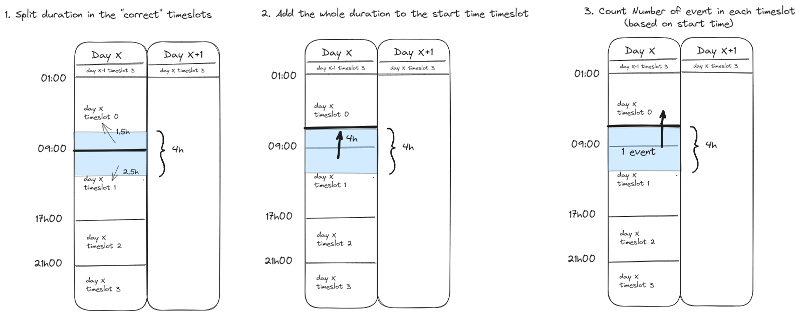
1. Split duration in the “correct” timeslots This approach means we split the duration of each event based on the time slot cut of times, so that for example if we have a 4h event that starts in timeslot 0 and ends in timeslot 1, then the time in timeslot 0 will be added to timeslot 0, and the remaining time will be added to the next timeslot.

pros

• More accurate when it comes to the amount of time each user is active in a given timeslot

cons

• doesn’t take into consideration how many “events” there are in the different timeslots (i.e. if a user has multiple events throughout the time slot, it will just sum up the active time)
• more complicated to implement

2. Add the whole duration to the start time timeslot Calculate the start time of the event and add the whole duration to that timeslot.

pros

• simpler than 1

cons

• doesn’t show the time spent active in each timeslot accurately, ex. if a user starts a 4h session 1min before timeslot x ends, the whole duration will be added to timeslot x, despite most of the duration actually being spent in the next timeslot.
• also doesn’t take into consideration how many “events” there are in the different timeslots.

3. Number of event in each timeslot Calculate the star time for each event and use that to calculate the number of events in a given timeslot.

pros

• simple to implement
• takes into consideration nr of events
• more closely models the label data (since the thing we wanna predict is wheter a user is active during a certain timeslot not how much time they spend active)

cons

• Doesn’t take into consideration duration (an event that is 1min is counted the same as one that’s 6h) (maybe possible to improve on this by also considering duration?)

(Among these three approaches, the most effective one was the third approach, which considers the number of events in each timeslot. This may be attributed to the fact that the prediction task primarily revolves around whether there is any activity during a given timeslot rather than the exact amount of time spent. By leveraging the count of events, this approach provides a simplified yet meaningful representation of user engagement during specific time intervals.)

For approach 2 the goal was to extract features based on the content. taking into consideration the popularity of different shows, similarity in watching habits across users, generating embeddings for dramas based on their shared viewership patterns etc.

In short the following steps where followed:

1. Drama Popularity Metrics Calculation:
   • Total views, unique users, and average completion ratio for each drama are calculated from the training data.
2. Drama Connections Filtering Based on Shared Users:
   • The median number of shared users among dramas is used as a threshold.
   • Drama connections are established based on shared users.
   • Drama pairs with shared users meeting or exceeding the threshold are retained.
3. Drama Embeddings with DeepWalk Algorithm:
   • The filtered drama pairs are used to construct a graph.
   • The DeepWalk algorithm, implemented using Node2Vec, generates low-dimensional embeddings for dramas based on their shared viewership patterns.
   • Drama embeddings capture the underlying relationships for downstream tasks.
4. User-Level Feature Extraction:
   • User-level features like total played duration, total views, and unique dramas watched are aggregated from the training data.
5. Merging Features and Data:
   • User and drama features are merged with the original training data using relevant identifiers.
6. Merging Drama Embeddings:
   • Drama embeddings are merged with the training data based on drama identifiers.
7. Data Formatting:
   • The final dataset is organized with one row per user, containing user-level features and associated drama features.

A more detailed overview of the steps taken (as well as the code used) to generate all of the different features can be found here: GitHub - Alexnder77/-IE5054-: Some of my code for the NTU course 資料分析方法 (IE5054)

When it comes to my approach to trying out different models, tuning them and evaluating their performance, in essence the following steps where taken for both features:

1. Selecting the features to use
2. Separating the train data into train and validation set (using a 70-30 split)
3. Training and evaluating the base-model (compare against benchmark)
4. if the model did well, continue to hyperparameter tuning, trying to improve the score.
5. if the score gets high enough use it to make predictions on the test data

To establish a good benchmark test the light data was used with a XGB model, after tweaking the model parameters a little succeeded in reaching an AUC score of 0.80833. This benchmark was later used to evaluate the performance of my other models with the custom features.

(Note: After the completion of the challenge, when the teams where presenting our work in class the wining team (Ying Train Yi Fa NTU 111-2 Data Analytics Term Project | Kaggle) succeeded in getting a score of 0.83957 just from the light data using XGB and the right hyperparameters)

Score: 0.82589

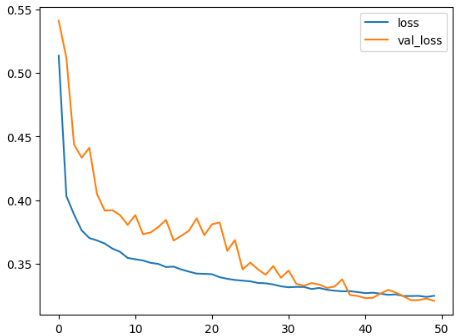
The Convolutional Neural Network (CNN) model is a deep learning architecture particularly effective in processing grid-like data, such as images or sequences. For the time-based features, the data was reshaped to take advantage of this to represent each user’s engagement across different time slots as a sequence.

The model consists of multiple convolutional and pooling layers, which can learn relevant patterns from the sequential data. These patterns can capture user behaviors like peak engagement times during certain days or time intervals. The final dense layers with a sigmoid activation function output probabilities of user activity during each time slot. By training this model on your time-based feature data, it can learn to recognize temporal patterns in users’ viewing schedules and predict their engagement in different time slots.

 1
 2
 3
 4
 5
 6
 7
 8
 9
10
11
12
13
14
15
16
17
18
19
20
21
22
23
24
25
26
27
28
29

model = Sequential()

model.add(Conv2D(64, 3, activation='relu', padding='same', input_shape=[32, 32, 1]))
model.add(MaxPooling2D(pool_size=(2, 2)))
model.add(Dropout(0.25))
model.add(BatchNormalization())

model.add(Conv2D(128, 3, activation='relu', padding='same'))
model.add(MaxPooling2D(pool_size=(2, 2)))
model.add(Dropout(0.25))
model.add(BatchNormalization())

model.add(Conv2D(256, 3, activation='relu', padding='same'))
model.add(MaxPooling2D(pool_size=(2, 2)))
model.add(Dropout(0.25))
model.add(BatchNormalization())

model.add(Conv2D(512, 3, activation='relu', padding='same'))
model.add(MaxPooling2D(pool_size=(2, 2)))
model.add(Dropout(0.25))
model.add(BatchNormalization())

  
model.add(Flatten())
model.add(Dense(512, activation='relu'))
model.add(Dropout(0.5))
model.add(Dense(256, activation='relu'))
model.add(Dropout(0.5))
model.add(Dense(28, activation='sigmoid'))

 1
 2
 3
 4
 5
 6
 7
 8
 9
10
11
12
13
14
15

model.compile(loss='binary_crossentropy',
             optimizer='adam',
             metrics=['accuracy'])

model.fit(X_train, y_train,
          batch_size=1024, #128
          epochs=50,
          verbose=1,
          callbacks=[plot_losses],
          validation_data=(X_val, y_val))

  
score = model.evaluate(X_test, y_test, verbose=0)
print('Test loss:', score[0])
print('Test accuracy:', score[1])

Score: 0.82664

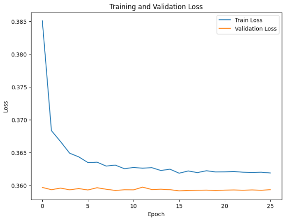
This model was used to try to combine the advantages of CNN and LSTM (Long Short-Term Memory). Which should be especially suited for modeling sequential data with spatial patterns

The CNN layers extract local patterns from the sequence, while the LSTM layers capture longer-term dependencies.

 1
 2
 3
 4
 5
 6
 7
 8
 9
10
11
12
13
14
15
16
17
18
19
20
21
22
23
24
25
26
27
28
29
30
31
32
33
34
35

model = Sequential()
model.add(Conv2D(64, 3, activation='relu', padding='same', input_shape=[32, 32, 1]))
model.add(Conv2D(64, 3, activation='relu', padding='same'))
model.add(MaxPooling2D(pool_size=(2, 2)))
model.add(BatchNormalization())
model.add(Dropout(0.25))

model.add(Conv2D(128, 3, activation='relu', padding='same'))
model.add(Conv2D(128, 3, activation='relu', padding='same'))
model.add(MaxPooling2D(pool_size=(2, 2)))
model.add(BatchNormalization())
model.add(Dropout(0.25))

model.add(Conv2D(256, 3, activation='relu', padding='same'))
model.add(Conv2D(256, 3, activation='relu', padding='same'))
model.add(MaxPooling2D(pool_size=(2, 2)))
model.add(BatchNormalization())
model.add(Dropout(0.25))

model.add(Conv2D(512, 3, activation='relu', padding='same'))
model.add(Conv2D(512, 3, activation='relu', padding='same'))
model.add(MaxPooling2D(pool_size=(2, 2)))
model.add(BatchNormalization())
model.add(Dropout(0.25))

#LSTM layers
model.add(TimeDistributed(Flatten()))
model.add(LSTM(256, return_sequences=True))
model.add(LSTM(256))

model.add(Dense(512, activation='relu'))
model.add(Dropout(0.5))
model.add(Dense(256, activation='relu'))
model.add(Dropout(0.5))
model.add(Dense(28, activation='sigmoid'))

SCORE 0.83112

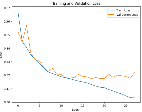
parameter values:

 1
 2
 3
 4
 5
 6
 7
 8
 9
10
11
12
13
14
15
16
17
18
19

params = {
    'objective': 'binary:logistic',
    'eval_metric': 'logloss',
    'eta': 0.1,
    'max_depth': 5,
    'subsample': 0.8,
    'colsample_bytree': 0.8,
    'lambda': 1,
    'alpha': 0
}
  
# Train the XGBoost model with early stopping
model = xgb.train(
    params,
    dtrain,
    num_boost_round=1000,
    evals=[(dtest, 'eval')],
    early_stopping_rounds=10
)

Two different Ensemble learning techniques was used to try to improve the score further. these techniques being weighted averaging and stacking.

Averaging in ensemble learning refers to combining the predictions of different models by simply taking the average of the predictions. in theory this can improve the result since some models ex. LSTM might be good at predicting certain time related features where as CNN or XGB might be better at predicting other relationships. So in theory by combining the different models we can take advantage of the strengths of different models at the same time.

The simplest way to do that is through simply averaging the predictions, another usually better way is to use weighted averaging by applying a weight to the different predictions.

So if we have the above mentioned models and they generate the predictions: $P_1 , P_2 \text{ and } P_3$ we get the weighted average (WA) by applying the weights $w_1, w_2, w_3$ like this: $$WA = \frac{w_1P_1+w_2P_2+w_3P_3}{3} $$

Different weights where tried and the best combination came from combining the above 3 models with the weights: 0.4 (XGB), 0.3 (CNN) and 0.3 (CNN + LSTM) -> Score: 0.836

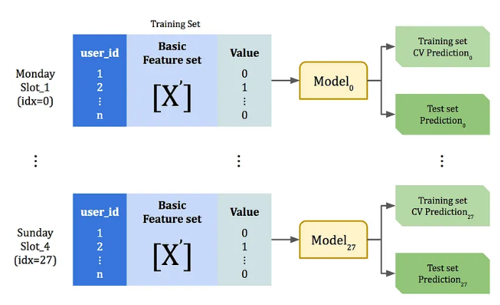
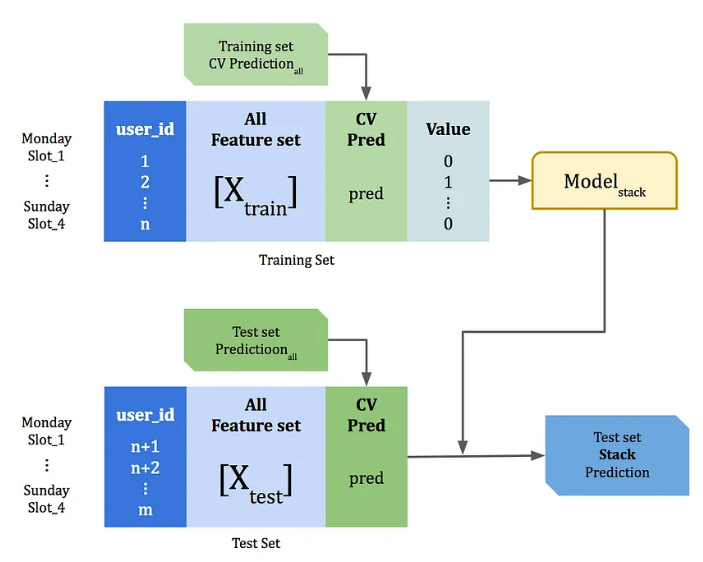
A more advanced ensemble stacking approach was also tried, based on Kaishen Tseng’s work

source: KKTV Data Game-17.11 1st Place Solution | by Kaishen Tseng | Medium

In short, 28 different base-models where created, one for each timeslot to be predicted. These models are trained on a subset of the train data then used to generate both train set and test set predictions.

source: KKTV Data Game-17.11 1st Place Solution | by Kaishen Tseng | Medium

The train set predictions are then added to the input features (of the train set) and used to train the Stack model. This stack model is then used to make the final prediction on the test data combined with the test predictions from the previous base models.

Applying this stacking method was a lot more work than the previous methods, but for some reason the score didn’t improve.

This was my first Kaggle challenge and it was a lot of fun, even though my team’s leaderboard position might not have been at the top, I’m genuinely content with our achievements and the knowledge gained throughout the project.

Some Thoughts:

The Content based features didn’t score very well, its likely that there is a mistake somewhere, maybe in generating the “Drama Embeddings” since its hard to tell what these values mean once they are generated.

the team that won the challenge did so using the light data set, meaning that its possible to get a very good score using that.

1. Learning Opportunity: Engaging in this Kaggle competition allowed me to delve into real-world data challenges, learning valuable lessons in data preprocessing, feature engineering, and model selection.

2. Feature Pitfall: Although we experimented with content-based features, they didn’t yield satisfactory results. The issue might lie in the process of generating “Drama Embeddings,” which proved challenging to interpret.

3. Light Data Triumph: Interestingly, the winning team based their model on only the light data set (with a score of 0.83957). This underscores the fact that with clever strategies and feature utilization, good results can be achieved even with more limited data.

   This also makes me wonder if a better score is achievable using my features with their model (since my features should contain more data)

In retrospect, this experience not only expanded my practical data science skills but also deepened my understanding of the iterative nature of problem-solving in a competitive setting. I’m looking forward to trying more challenges like this in the future.